Parameter Sweeping and Visualisation

Parameter sweeping systematically explores a grid of candidate parameter values and identifies the combination that best reproduces the observed data. In nlmixr2autoinit, this approach is used to derive initial estimates for model structures that cannot be solved analytically from one-compartment PK analysis, specifically:

Multi-compartment models (2-compartment and 3-compartment)
Nonlinear elimination models (Michaelis-Menten kinetics: $V_{max}$ and $K_m$ )

This vignette explains how to run parameter sweeping independently and how to visualise the sweep results to understand the parameter space.

Running Parameter Sweeping

We can bypass the automated base parameter calculation from nlmixr2autoinit and instead specify $CL$ , $V_d$ , and $K_a$ directly. This is useful when we are only interested in exploring the complex model parameters such as $V_{max}$ and $K_m$ , without re-running the full estimation pipeline.

For example, sim_sens_1cmpt_mm() then performs the sweep for $V_{max}$ and $K_m$ in a one-compartment model with Michaelis-Menten elimination for IV data.

library(nlmixr2autoinit)
#> Loading required package: nlmixr2data
# Example: IV dosing scenario with automatic Vmax and Km
out1 <- sim_sens_1cmpt_mm(
  dat    = Bolus_1CPTMM,
  sim_vmax = list(mode = "manual", values = c(200, 400, 600, 800, 1000, 1200)),
  sim_km   = list(mode = "manual", values = c(5, 10, 50, 100, 200, 400)),
  sim_vd   = list(mode = "manual", values = 70),
  sim_ka   = list(mode = "manual", values = NA),
  route = "iv"
)

We can inspect the first few rows of the simulated output and see that multiple goodness-of-fit metrics are returned for each parameter combination. Definitions of these metrics are provided in ?metrics..

Here we focus on rRMSE2, the symmetric relative root mean squared error, which normalizes each predicted–observed difference by the mean of the predicted-observed pair and is used here to compare parameter sets.

head(out1)
#> # A tibble: 6 × 11
#>    Vmax    Km    Vd    Ka      APE   MAE  MAPE  RMSE rRMSE1 rRMSE2
#>   <dbl> <dbl> <dbl> <dbl>    <dbl> <dbl> <dbl> <dbl>  <dbl>  <dbl>
#> 1   200     5    70    NA 5572697.  802.  608. 1400.   87.9   73.9
#> 2   200    10    70    NA 5594331.  805.  621. 1402.   88.0   73.6
#> 3   200    50    70    NA 5753722.  828.  729. 1413.   88.8   76.8
#> 4   200   100    70    NA 5899008.  849.  821. 1425.   89.5   79.3
#> 5   200   200    70    NA 6096946.  877.  933. 1443.   90.6   81.9
#> 6   200   400    70    NA 6344339   913. 1059. 1468.   92.2   84.4
#> # ℹ 1 more variable: Cumulative.Time.Sec <dbl>
# # A tibble: 6 × 11
#    Vmax    Km    Vd    Ka      APE   MAE  MAPE  RMSE rRMSE1 rRMSE2 Cumulative.Time.Sec
#   <dbl> <dbl> <dbl> <dbl>    <dbl> <dbl> <dbl> <dbl>  <dbl>  <dbl>               <dbl>
# 1   200     5    70    NA 5572697.  802.  608. 1400.   87.9   73.9                0.33
# 2   200    10    70    NA 5594331.  805.  621. 1402.   88.0   73.6                0.64
# 3   200    50    70    NA 5753722.  828.  729. 1413.   88.8   76.8                0.99
# 4   200   100    70    NA 5899008.  849.  821. 1425.   89.5   79.3                1.29
# 5   200   200    70    NA 6096946.  877.  933. 1443.   90.6   81.9                1.6 
# 6   200   400    70    NA 6344339   913. 1059. 1468.   92.2   84.4                1.92

Visualising Sweep Results

We can visualize the sweep results as a heatmap to examine how model fit changes across combinations of $V_{max}$ and $K_m$ , with lower rRMSE2 indicating better fit. In this example, the optimal parameter combination is identified at $V_{max}=1000 mg/h$ and $K_m=200 mg/L$ , which gives the lowest rRMSE2 among all tested values.

library(ggplot2)
best <- out1[which.min(out1$rRMSE2), ]
p1<-ggplot(out1, aes(x = factor(Vmax), y = factor(Km), fill = rRMSE2)) +
  geom_tile() +
  geom_tile(
    data = best,
    aes(x = factor(Vmax), y = factor(Km)),
    fill  = NA,
    color = "black",
    linewidth = 1.2
  ) +
  geom_text(aes(label = round(rRMSE2, 1)), size = 4.5, color = "grey20") +
  scale_fill_gradient(
    low  = "#1a9641",
    high = "#f7f7f7",
    name = "rRMSE2"
  ) +
  labs(
    x = expression(V[max]),
    y = expression(K[m])
  ) +
  theme_bw() +
  theme(
    axis.title = element_text(size = 11, face = "bold"),
    axis.text  = element_text(size = 10)
  )
print(p1)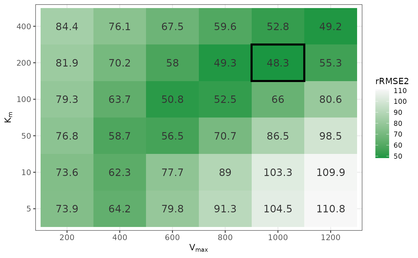

Running Parameter Sweeping

Visualising Sweep Results

See Also